一个系统的性能是由多方面共同作用的结果,当我们分析系统性能时,需要知晓主要的性能瓶颈点。本文从CPU调度,内存管理,文件系统,IO,网络等方面介绍了性能分析的注意点,并提供了一些工程上的建议。文中提到的Brendan Gregg是这方面的专家,建议阅读其相关文章。
原创文章版权归原作者所有,商业转载请联系原作者获取授权,任何转载请注明来源:https://xupifu.github.io/2017/04/27/system-performance/
1 CPU及调度
1.1 SMP和NUMA
SMP,Symmetrical Multi-Processing,对称多处理。
- 各物理CPU共享内存及总线结构,但有独立的Cache
- 每个物理CPU由多个Core组成,一般共享L2 Cache,有独立的L1 Cache
- 每个Core可以通过超线程(Hyper-threading)技术实现多个硬件线程,一般称为Virtual CPU,所有东西共享,包括L1 Cache
SMP架构的一个主要缺点是:内存及总线是共享的,多线程下的总线资源竞争会影响整系统的性能。
NUMA,Non Uniform Memory Access Architecture,非一致性内存访问。与SMP不同的地方在于,内存会被划分成多份本地内存,各物理CPU优先使用自己的本地内存,远端内存也可以使用,但代价相对比较大。这种架构的好处是,每个物理CPU有自己的内存控制器及内存区域,实际使用中,需要考虑将进程/线程限定在一定区域内,以降低资源的争抢,从而提高效率。
【蚍蜉】注:NUMA架构下的内存分配如果仅限制(或优先)在本地内存,则需要特别注意应用的分布,以免过于集中,导致内存管理成本增加(如swap活动过于活跃),从而影响系统性能。
实际不止有以上两种架构,但不论哪种,都需要考虑如何充分发挥多CPU的性能优势,不能让一些CPU太繁忙,另外一些又太空闲,即所谓的负载均衡。负载均衡意味着线程迁移,而线程迁移后,线程对应的各级Cache可能会无效,需要重填。而NUMA架构中,线程拥有的内存可能会从本地变成远端内存,内存访问时间将加大。这些迁移的代价需要在负载均衡处理中重点考虑,下节将介绍affinity,即亲和性的概念,负载均衡需要根据亲和性程度来决定是否迁移。
1.2 affinity
每个进程/线程都有自己的资源,尤其是运行过程中的临时资源,比如各级Cache,线程迁移后,如果对应的资源还能继续使用,则认为亲和度相对高一些。可见,除非逼不得已,否则线程应该尽量选择亲和度高的CPU进行迁移。
结合上节的介绍可知,Virtual CPU到Core再到物理CPU,各级资源的共享程度不同,线程迁移的代价也不同,越往上,代价越大。据此,内核开发人员Nick Piggin等人在Linux 2.6中引入了Scheduling Domains,即调度域的概念,如下图所示:
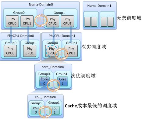
负载均衡算法就是建立在调度域的基础上的,当迁移代价越大时,应该加大线程迁移的阻力,甚至不做迁移。在/proc/sys/kernel/sched_domain中,可以设置一些参数,协助负载均衡算法进行决策。
除了自主的负载均衡,系统还提供系统调用(sched_setaffinity)和工具(taskset,numactl等),用于将进程/线程绑定在一定的调度域中。相比较系统的自主行为,用户更清楚自己的程序行为,可以由用户决定自己的调度域。
NUMA架构对操作系统和应用的要求比较高,程序编写尤其需要注意内存的分配,并防止内存由本地变成远端(线程迁移时,内存不会跟着迁移),因此还涉及到调度域的绑定。但无论怎样的设计,分布在不同域中的线程,如果互相之间还有资源共享,那么远端访问是避免不了的。因此,在实际使用中,是否启用NUMA还是需要慎重考虑的,可以在内核启动参数中通过添加”numa=off”关闭NUMA特性。
【蚍蜉】注:CPU0是一个特殊的CPU,比如中断处理,故一般不建议将进程绑定到该CPU上。
1.3 irqbalance
与进程/线程类似,中断处理需要结合CPU自身的架构,考虑处理的性能和CPU的功耗。一般情况下,中断处理集中在CPU0上,对于普通负载,这种处理方式没有问题,而且还可以节省其他CPU的功耗。但在较大负载的情况下,CPU0可能就存在瓶颈,再考虑到CPU架构,中断/线程处理最好是在自己就近的CPU上。理论上,将中断分散到合理的CPU上,是有利于性能的提高的。Linux系统中,irqbalance是一个后台服务,用来实现上述目标。具体实现中,最困难的是均衡处理的启动时机。irqbalance服务是通过周期性(比如10秒)的数据收集和统计分析,来判断这个时机的。不过,现有的统计分析算法可能会存在误判,从而导致不必要的自动迁移,影响系统性能的稳定性。
如果不想使用该功能,可以通过/proc/irq/N/smp_affinity进行CPU亲和性绑定(N为中断号),或者关闭irqbalance服务。在一些特殊场景中,比如高性能/高负载场景,可以考虑关闭该功能,让应用自己管理中断负载和分布。
1.4 cpufreq
CPU除了性能方面的考虑,功耗也是一个非常重要的指标,CPU一般通过变频功能来达到功耗控制的目的。CPU常见的模式包括performance(全速),powersave(低功耗),ondemand(按需)等。比如,对于有性能要求的应用,可通过以下方式将CPU调整到performance模式(也可以通过BIOS进行设置):
|
|
其中,cpufreq目录下还有一些其他信息和参数可供使用。
值得一提的是,Intel CPU的P-State特性可能导致以上的设置无效,即:就算在BIOS中关闭了变频功能(或者内核启动参数”intel_pstate=disable”),因功耗考虑,CPU内部依然可能保持变频。具体描述可见后文Arjan van de Ven的文章摘录。
1.5 优先级
优先级是系统进行进程调度的一个重要依据(调度器/策略请自行查阅相关文章)。进程一般可分为实时进程和非实时进程。实时进程有很强的调度需求,并且有一定的响应时间要求。除了自行切换或更高优先级的进程出现,实时进程通常不允许被抢占。非实时进程大致又可分为IO-Bound和CPU-Bound两种进程:
- 对于IO-Bound进程,由于大部分时间是在等待IO的,因此一旦可运行了,一般会赋予较高的运行优先级,这类进程通常是一些交互式的进程
- 对于CPU-Bound进程,通常主要是占用CPU,这类进程通常是一些后台服务或计算型进程
实际应用中,一般无法严格区分进程到底是IO-Bound还是CPU-Bound,两者可能是混合在一起的。
一般系统都会提供系统调用或工具(nice/renice),让用户设置自己的任务优先级。
工程建议:对关键进程,可适当提高优先级,对非关键进程,可考虑降低优先级。在专用系统中,一般不涉及其他服务(进程),故不必过多考虑优先级调整,使用默认即可。
1.6 CPU使用情况
Linux中,CPU的使用情况被分成了以下几类:
- 占用率:一般分为user,system,idle,iowait等占用比例
- 中断发生的次数,其处理时间归入system类
- 上下文切换次数,触发因素一般为锁竞争等,其处理时间归入system类
- 运行/阻塞的进程数,结合CPU占用率分析阻塞原因,如占用率不高,则可能为其他因素(比如IO)导致。一般情况下,每CPU不宜有太多进程(工程建议:2-3个)
【蚍蜉】注:锁竞争,线程迁移导致的Cache代价等,是目前多CPU性能无法充分发挥(随CPU数线性增长)的重要因素。
2 内存/缓存
2.1 内存分配
这里的内存分配主要指的是用户空间下的内存分配,常见的API有malloc/realloc/calloc等。对于经常性的进行动态分配的应用,随着时间的增长,内存的碎片化会越来越严重。因此,在一些情况下,可能导致这些API性能极其低下。一般的解决方法是:在用户空间维护一系列不同尺寸的内存池,尽可能绕过内核的页面管理。目前,已经有一些替代库(如tcmalloc)可以提供此类功能,建议程序使用。
2.2 HugePage
HugePage是Linux内核上一种使用内存块的方法。相比较传统的4K页,优点是能够降低页面管理的开销,比如页表大小,同时HugePage不允许换出,通过锁定内存,可以避免因swap导致的性能稳定问题。工程实践中,在内存较大的环境中,HugePage作用比较明显,对于小内存环境,则作用一般。通常,HugePage需要预留内存,这可能导致内存浪费。后来的Transparent HugePage特性,可以动态分配,无需预留,不过,该特性还需要一定的稳定时间。Linux下,可以通过sysctl设置”vm.nr_hugepages”,具体数值需要结合业务应用进行设置。
2.3 内核高速缓存
Linux内核提供的高速缓存(Page Cache)是一个通用的实现,对于大部分的应用场景是非常有效的,但缺点也同样明显,对于一些特殊应用,使用Page Cache反而影响应用性能。因此,这些应用一般都选择跳过Page Cache,自己管理缓存。
这里,仅给出Linux的高速缓存的几个注意点:
- 回写策略采用writeback方式,存在数据丢失的风险
- 对于写入量较大的应用,容易导致脏页率过高,从而阻塞写操作。这种情况下,不能完全依赖缓存的自动回写机制,应用需在合适时机触发回写操作,以免脏页率过高影响应用的使用
- 页缓存使用了预读,对于局部性较好的应用(比如顺序读居多),该项功能非常有效,但对于随机读的应用,反而会影响性能,可以通过设置关闭预读功能,或者直接使用Direct IO访问方式
- 替换策略是由页面回收配合完成的,其中包含了swap的换进换出,会引发IO读写,可能造成性能的不稳定,一般建议关闭(通过sysctl设置”vm.swappiness=0”)
- 页缓存的各种机制和策略是针对整系统的,而不是某个应用,其效用受外界因素的影响较大。对于有性能要求的应用,最好不要依赖于Page Cache,而是自己实现和管理缓存
- 页缓存理论上可以用来加速所有的块设备,但最早主要是针对磁盘特性进行设计的,对于新的一些存储设备,这些设计就不一定能够很好的使用新设备的特性
- 在/proc/sys/vm中有一些影响系统性能的参数可供调节
2.4 内存使用情况
Linux下提供了free/vmstat等工具,可以查看内存剩余,swap活动,缺页异常数量等情况,有性能要求的应用,应规划好内存大小,尽量降低甚至规避swap和页面回收的影响。工程建议:应用可用的内存不低于物理内存的20%。
3 文件系统
- 块大小:通常在创建文件系统时指定,可以根据文件大小的分布进行设置,文件较大时可采用较大的块获取较高性能,文件较小时可取小值以减少空间浪费
- 日志模式:现在的文件系统大部分都具有日志功能,日志工作模式主要有(mount文件系统时指定):
- journal:数据和元数据均写入日志区,数据保证最好,但性能最差
- writeback:只有元数据写入,不保证顺序,不保证数据一致性,但性能最好
- ordered:只有元数据写入,要求保证顺序,介于以上两者之间,一般采用该模式
- 文件数量限制:一般系统会有打开文件数量的限制,Linux下可通过ulimit修改,ulimit还可设置最大进程数,堆栈大小等资源限制
- barrier:一些硬盘具有write cache功能,对于有顺序要求的写操作,一般需要先发送barrier命令将cache刷回到物理介质上,以免出现写乱序导致的数据一致性问题。对于有掉电保护功能的设备,可关闭该功能以提高读写性能(mount文件系统时指定,nobarrier)
- 访问时间:文件被创建,修改和访问时,系统会记录这些时间信息。如果存在较多的读文件操作,频繁记录访问时间是一笔不少的开销。而在大部分情况下,用户是不太关心访问时间的。因此,可在mount文件系统时关闭该功能(noatime,nodiratime)
- TRIM:这是SSD专用的特性,用来通知SSD哪些页面不再使用,可以辅助SSD进行垃圾收集,使用该功能需注意支持的成熟度,可在mount文件系统时指定(discard)
4 存储IO
4.1 IO访问
系统提供的IO访问方式非常多,初步可分类为映射式IO和拷贝式IO。映射式IO对应有系统调用mmap,拷贝式IO对应的系统调用有read/write,pread/pwrite等。在拷贝式的IO中,又有一些标志位可以设置以启动相应功能,比如O_NONBLOCK标志位,表示IO是否阻塞,O_DIRECT标志位则表示IO是Direct IO还是Buffer IO(即是否经过Page Cache)。以上IO一般指的都是同步IO,即当时等待IO返回,为了更加有效的利用CPU,系统还提供异步IO访问方式,线程不必等待IO结束,可以转做其他任务。
事件通知方面,系统提供了Multiplexing IO技术,即多路复用IO技术,可以用来监听多个文件/套接字的内容变化情况,之后对相应的文件/套接字进行处理。常见的系统调用有select/poll/epoll。该技术在高性能网络服务器中应用非常广泛。
高性能场景,一般使用epoll和异步IO的组合。对于随机IO或自有缓存管理的应用,还建议使用Direct IO方式绕过Page Cache。
4.2 内核IO调度器
Linux内核中的IO调度器主要包括Deadline,CFQ,AS(Anticipatory)和NOOP。根据一些工程经验,SATA/SAS硬盘建议使用Deadline调度器,普通SSD硬盘建议使用NOOP调度器,NVMe/PCIe的SSD则不必设置,一般由驱动或内部管理直接完成调度。关于IO调度器,公开资源较多,此处不赘述。
设置方式示例如下:
|
|
也可在启动参数中指定,比如”elevator=deadline”。
4.3 IO性能
IO性能主要包括IOPS(每秒IO数量),Throughput(吞吐量),Latency(延迟/响应时间)。分析IO性能时,需注意IO队列深度的情况,比如阻塞的IO数等。查看和分析IO情况的工具有iostat,blktrace,fio等。
5 网络
网络分析和调优是一个非常庞杂的话题,已超出本文作者能力,此处仅提供几个简单的点:
- 网络带宽:是否为瓶颈
- 连接池:创建连接是需要开销的,同时需要占用文件描述符,对于频繁的短连接请求,不断的创建/销毁是不必要的,可以将连接池化,即维持一些连接,节省创建时间。目录/proc/sys/net/ipv4下有相关参数可设置(也可通过sysctl)
- 使用多路复用技术
- 其他如MTU,网卡缓冲区也可设置用来优化传输性能
6 相关工具
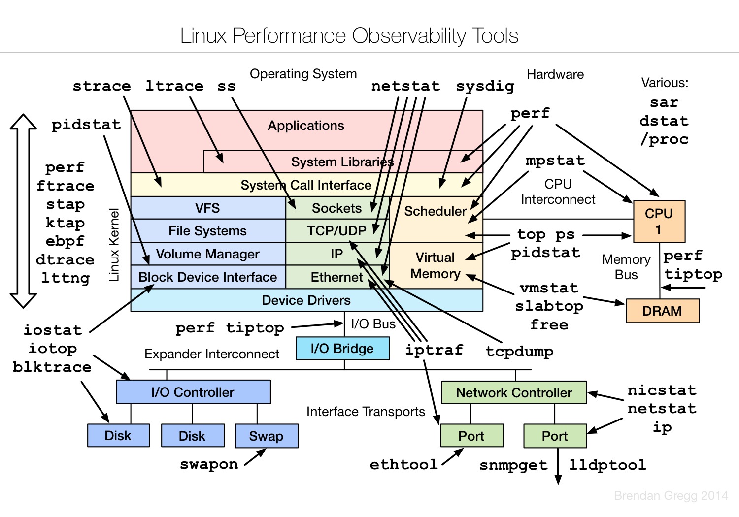
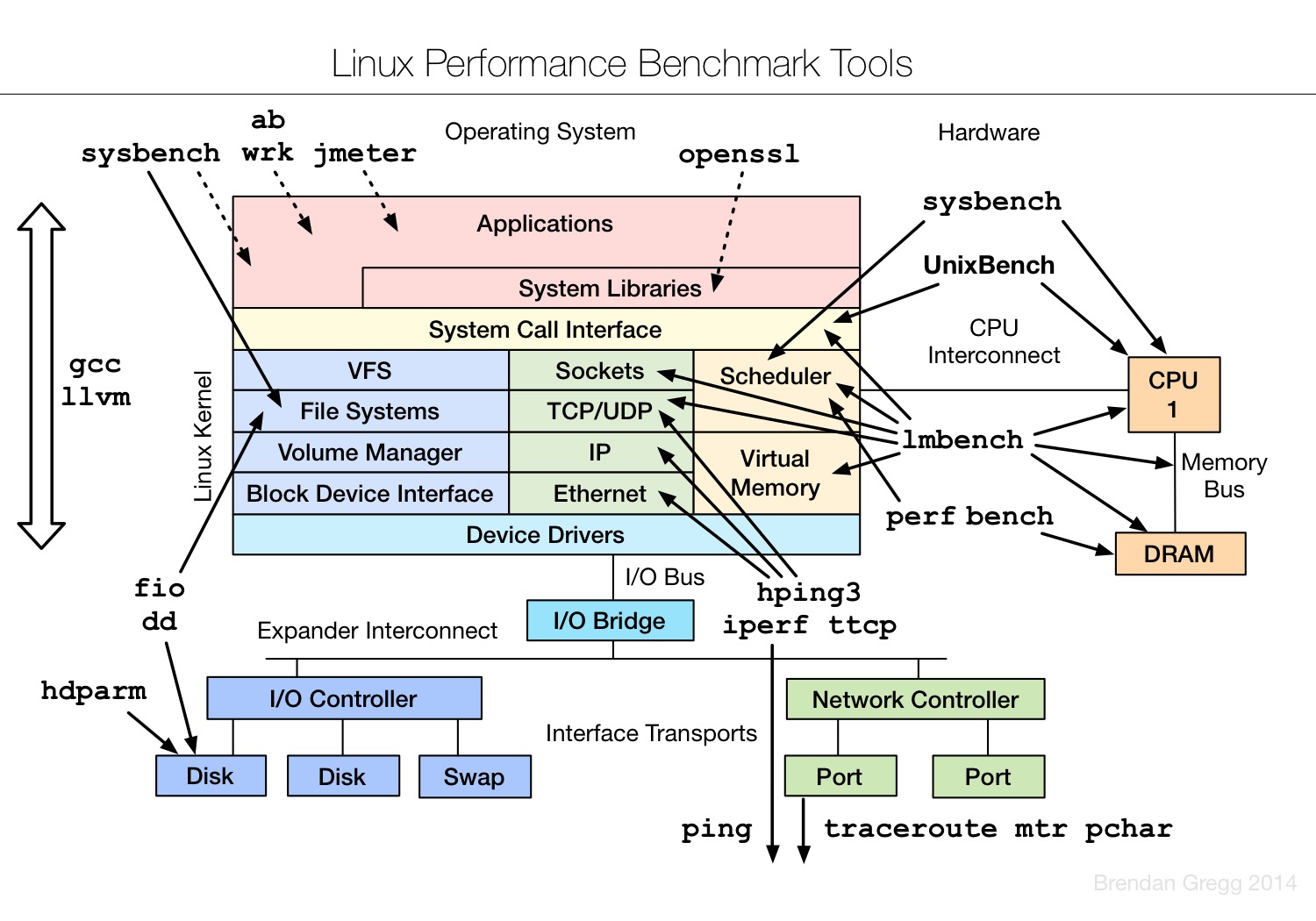
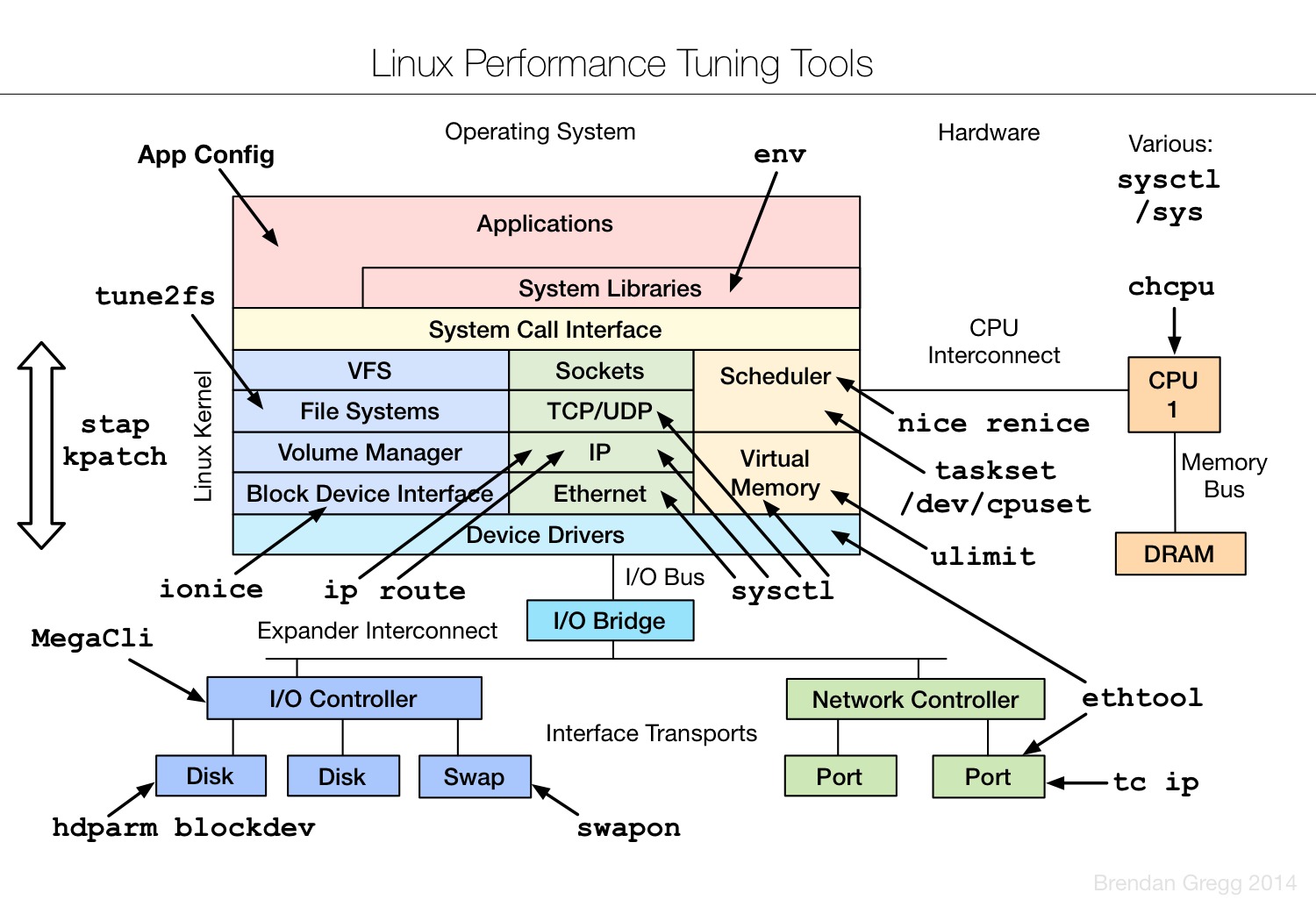
系统性能分析的方法及相关工具,可见该领域大牛Brendan Gregg的个人网站(附录1),诸多Linux系统下的性能监控和数据采集分析等工具均出自该人。Linux Performance Analysis and Tools为其曾经的演讲主题,强烈建议阅读。本节仅列出几张图片,可结合上文介绍的注意点进行理解。
7 小结
本文涉及了系统层面主要的一些性能点,包括CPU调度,内存,文件系统,IO和网络。对于一个系统或应用,是否存在瓶颈,可以通过以上几个方面逐一排查。当然,除了系统层面对性能的影响,应用本身的优化也是非常关键的。由于应用类型非常多,本文无法展开叙述,一般可以从代码,算法,业务逻辑,架构等方面进行相应的优化考虑。
附录
- Brendan Gregg. Linux Performance Analysis and Tools
- Arjan van de Ven. Some basics on CPU P states on Intel processors
- irqbalance
附:Some basics on CPU P states on Intel processors
by Arjan van de Ven
There seems to be a lot of things people don’t realize on how P state selection works on Intel processors, and arguably the documentation is slightly confusing in this regard… and things have been changing generation to generation.
First, why use the word “P state” and not “frequency”? This is important in terms of thinking about how this works.
“Clock frequency” is something that you measure over some period of time, basically an average on how fast a clock signal went up/down. It’s something you can measure, but it’s backwards looking. Intel CPUs expose two counters (aperf and mperf) via MSR registers, and if you look at these two registers at two separate times (far enough apart to avoid rounding effects), the ratio of the delta in these two registers gives you a very nice “average frequency” over your measurement interval. (The official SDM documentation has the exact formula for this)
A P state is a number the OS tells the hardware regarding how much performance it would like to see on a certain (logical) cpu; a P state request is very much something forward looking.
So how are these related?
In the ten year old, single core, no hyperthreading world, things were relatively simple. You could basically map a P state to some “frequency” that you’d get, and as the marketing folks told us, a higher frequency means more performance.
Today, things are much more complex in several key ways.
First of all, and this is important and different from 10 years ago… no matter which P state you ask for, when a logical processor is idle (C state), its frequency is typically 0. The exception to this “typically” is the lightest of the C states (C1), where the frequency is the lowest frequency the CPU supports, and not zero. (but going into C1 is pretty rare, and very short lived, so for this posting, I’m going to ignore C1).
A second important aspect is that of “coordination”. For practical reasons, on current Intel processors, all the cores in a package share the same voltage. And because running at a lower frequency than possible at a certain voltage is inefficient, all the cores will also share the same clock frequency at any one time. Of course, except the cores that are idle, because their frequency is zero!
Because the OS will ask each individual logical processor for a separate P state, some reconciliation is needed between the different cores. This reconciliation is actually very simple, at any point in time, the frequency of all the cores is the maximum of what each of the individual cores wants. Of course, minus the idle cores. Their frequency is zero, and the maximum of “something” and “zero” is “something”.
A simple example is appropriate here.
Lets take a two core system (core A and core B, that are initially both busy).
Core A would want to have a clock that ticks at 1 Ghz, and Core B wants a clock that ticks at 2 Ghz.
The maximum of 1Ghz and 2Ghz is .. 2Ghz, so Core A and Core B will both run at 2 Ghz, even though core A only asked for 1 Ghz.
But now at time X, Core B is going idle. Since an idle core has a frequency of zero, and the maximum of zero and 1Ghz is 1Ghz… Core A now runs with a clock of 1 Ghz.
The key thing here is that Core A gets a very variable behavior, independent of what it asked for, due to what Core B is doing.
Or in other words, the forward predictive value of a P state selection on a logical CPU is rather limited.
Sound complex? Now imagine that the GPU on die is in many ways like a CPU core…. and realize that what I described above is actually a simplification of reality.
Another development in the last few years has been that of “Turbo”.
Some people call it “overclocking”, but it isn’t overclocking, it’s all within the specs of the hardware. Turbo exists because in a multi-core system, it’s possible to run a single core faster than the frequency that is on the label of the box when you buy the processor. This has to do with power budgets; when you buy a 35 Watt TDP cpu, the CPU isn’t supposed to use more than 35 Watts. So if you have, say, 4 cores, that means each core by itself can use a little less than 9 Watts to fit that budget.
But if 3 of the 4 cores are idle… the one remaining core can use the whole 35 Watts. (Now add in that the GPU also counts into this 35 Watts as do several other shared resources, and it gets much more complex).
If this single core would be limited to 9 Watts instead of the full 35W even when the others are idle, a lot of potential performance is left on the table.
Now in the first processors that supported Turbo, the available “extra range” was limited, but this range has been growing and growing as core counts have gone up, power sensors have been added to the CPU and power levels have come down. (don’t be surprised to see that your CPU has more levels in the turbo range than it has outside the turbo range)
What does this mean? Well, when the OS asks for a P state value that is in the “Turbo Range”, it may not actually get the performance that maps to that level; the sum of the power in the system could be exceeding the allowed TDP value if that performance (clock frequency) was granted to all cores (remember from above that all running cores share clock frequency).
What you do get at any one point in time depends on what other cores and the GPU etc are doing…. and this will vary over time as cores go idle or become active, or as the GPU finishes a frame or starts a new complex frame… and even with temperature.
Or in other words, what frequency you get is highly dependent on other things including the C state selection policy and the graphics subsystem.
Another fun angle is that when a task is running completely memory bound, the performance of this task is basically independent of the clock frequency…. and some systems will detect this condition and temporarily lower the clock frequency to save power without reducing performance too much (all within the bounds of all the things I described above).
If it wasn’t clear yet, a lot of what I described above varies from generation to generation quite a bit… and its going to change quite a bit more in the next few years.
In the 3.9 kernel we’ve introduced a new controller driver for the P states, simply because the previous, 10+ year old algorithm wasn’t cutting it anymore; too much has changed. By making the driver CPU generation specific, we can now select and tune algorithms for each specific generation, and do significantly better (30%+) than when we used a very generic algorithm.
Another thing to realize from all of this is that while it’s easy to talk and look at performance looking backwards (aperf/mperf allow us to do that), predicting performance going forward, even if you are very deliberately picking a P state value, is often near impossible since what you will actually get depends a LOT on what the other parts of the system are doing.